
Why Design Conditions Hide the Real Operating Cost
Design conditions describe a chiller plant at one idealized moment. Peak load sets the maximum cooling the building is expected to need. A stated entering condenser water temperature pins the heat-rejection side of the equation, usually at a favorable value such as 85 degrees F. Full-load kW/ton says how much power the machine draws to deliver that peak tonnage under those fixed inputs. The three numbers together make a snapshot that is easy to specify, compare, and certify.
That snapshot has become the dominant selection and compliance benchmark. Engineers size equipment against it, manufacturers publish it, and codes and utility rebates reward it. Standardization lets it travel cleanly across bids and submittals, which is why it attracts so much attention.
The benchmark describes a condition the building rarely occupies. Most facilities reach peak load for only a small fraction of their annual cooling hours; the rest is partial load, often well below half of design capacity. A chiller that looks efficient on paper at full load can lose much of that advantage as its part-load ratio falls and the machine cycles, unloads, or runs at poor compressor lift.
The metric that gets specified rarely matches the metric that gets experienced. Operating cost accumulates across thousands of off-peak hours, not the handful of peak ones, and full-load efficiency speaks to only a narrow slice of that. Design conditions optimize a single point; operating cost is the area under a curve. Until specifications weight part-load performance and reflect real condenser water temperatures and load profiles, the numbers that win the project will keep diverging from the dollars on the utility bill.
The two families of metrics are easy to confuse, and the one you quote at the ribbon-cutting is rarely the one that decides the bill. Design-point figures describe a single generous snapshot; part-load and annualized figures describe how the machine actually runs. The table below sets them side by side and shows what each measures, what conditions it assumes, and what it leaves out of the operating-cost picture.
Table: What design-point metrics promise versus what part-load and annualized metrics reveal about real chiller operating cost
| Metric | What It Measures | Typical Conditions | What It Hides About Operating Cost |
|---|---|---|---|
| Full-load kW/ton | Efficiency at 100% capacity, one operating point | AHRI 550/590 standard rating, 44 F chilled water, 85 F condenser water | Says nothing about the 90%+ of hours a chiller runs below full load |
| IPLV | Weighted efficiency across four load points (100%, 75%, 50%, 25%) | Standard AHRI 550/590 weighting, one set of fixed temperatures | Uses generic weights and a fixed condenser temperature that may not match your climate or lift |
| NPLV | IPLV-style weighting at your project’s design temperatures | Non-standard entering conditions defined by the engineer | Still a single weighted number; ignores hour-by-hour weather and load shape |
| IPLV applied at off-design conditions | Part-load efficiency recalculated as actual lift and temperatures move away from the AHRI test point | Site condenser and chilled-water temperatures across the year | Still one weighted number; no chiller sequencing or staging effects |
| Annualized energy use | Total kWh consumed across a full year of operation | Site weather, load profile, staging, and control strategy | Nothing; this is the bottom-line cost number, though it depends on modeling assumptions |
Read left to right and each column moves closer to the number on the invoice. A single full-load rating is an advertisement. An annualized energy figure built from your own load profile and weather file is a forecast you can take to the CFO. The gap between them is where surprise utility bills come from.
Defining Part-Load Efficiency Concepts
A chiller almost never operates at the condition stamped on its nameplate, which is why part-load efficiency matters more than any design figure in a submittal. Design conditions – full capacity, a specific condenser water temperature, a specific leaving chilled water temperature – describe the peak the plant must survive on the hottest afternoon of the year. For the thousands of hours in between, the machine is unloaded, cycling, and running far from its rated point, and that is where most of its energy is consumed.
Reading a chiller’s real operating cost takes a shared vocabulary. The terms below do most of the work.
- Load Ratio (Part-Load Ratio) – actual cooling output divided by design output, usually a percentage. A chiller serving 400 of its 800 rated tons sits at a 50% load ratio.
- kW/ton – electrical input in kilowatts per ton of cooling delivered. Lower is better, and it changes continuously with load and condenser conditions.
- IPLV – the Integrated Part-Load Value, a single weighted number (per AHRI 550/590) that blends efficiency at 100%, 75%, 50%, and 25% load using standard AHRI weighting and a fixed reference condenser temperature.
- NPLV – the Non-Standard Part-Load Value, the same weighting method applied to the actual condenser water temperature and operating conditions your project specifies instead of the AHRI defaults.
- Condenser Water Reset – lowering the entering condenser water temperature as load falls and wet-bulb drops, which reduces compressor lift and recovers efficiency at part load.
- Staging – sequencing multiple chillers (or compressor stages) on and off so each machine runs near its efficient range instead of one unit limping along at a low load ratio.
How unloading and staging move kW/ton
As load drops, compressors unload: screw and centrifugal machines slide or modulate capacity, while scroll and reciprocating units switch stages. A well-tuned chiller’s kW/ton improves as it leaves full load, reaching a minimum somewhere between roughly 50% and 70% of capacity, where compressor, heat exchangers, and controls work well together. Push down toward 20% or lower and the curve bends back up: fixed parasitic loads, oil and refrigerant pump energy, and reduced heat-exchanger velocity all inflate kW/ton.
Why 0.55 kW/ton is not the whole story
Picture a chiller selected at 0.55 kW/ton at design. During a mild shoulder-season week it may run at a 30% load ratio, where real efficiency could be 0.62 kW/ton or worse – about 13% more energy per ton than the specification sheet implies. Multiply that penalty across the thousands of hours the plant spends below 50% load and annual consumption diverges sharply from a design-only estimate. This is the gap IPLV and NPLV exist to expose. A strong IPLV says the machine is efficient across the part-load range; an NPLV recalculated with your condenser conditions says whether your staging strategy and reset schedule let it stay there. Judge a chiller by how it behaves for most of its running hours, not by the single point at 100%.
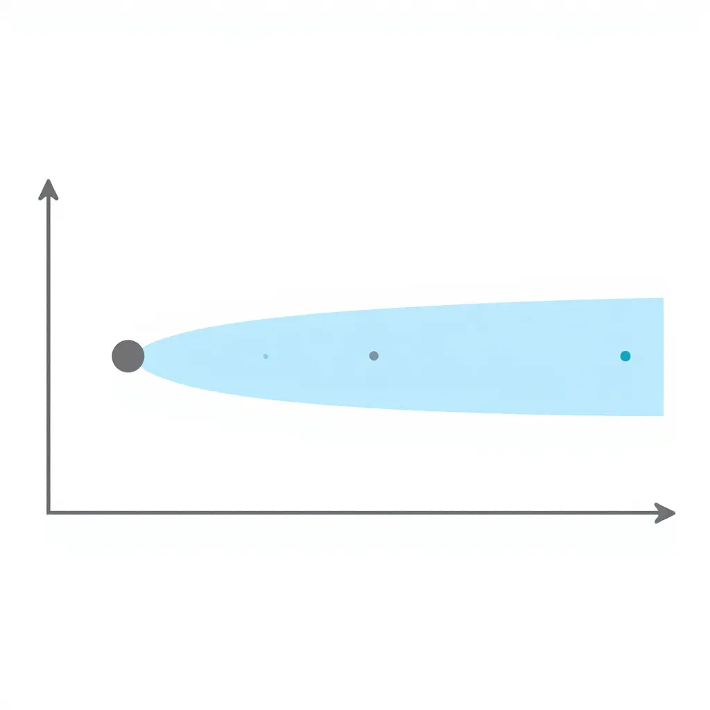
This diagram captures the problem. On the left, a single circle is the design point: the narrow set of conditions (peak load, one entering water temperature, full flow) that equipment is selected and rated around. On the right, the translucent band is the part-load operating band, the much larger range of conditions a plant actually runs in. The distance between the dot and the band is the point: selecting for a single design point tells you almost nothing about what you pay across a cooling season, when the plant is cycling, staging, and unloading.
What Drives Part-Load Losses
Chillers rarely run at nameplate conditions. Most of the year they sit between 20% and 70% load, which is where part-load efficiency drains the budget. The factors below erode performance and raise operating cost.
-
Oversized chillers that cycle instead of modulate.
An oversized machine reaches setpoint fast, then shuts off. It cannot throttle down smoothly, so it cycles all day, and every restart burns extra energy and wears the compressor. Design load rarely matches real load. -
Condenser approach degradation.
When the condenser approach widens, the chiller works harder to reject the same heat. Fouled tubes and scaling are the usual causes, and a few degrees of lost approach can add double-digit energy penalties. -
Cooling tower and pump energy penalties.
Tower fans and condenser pumps often run at fixed speed regardless of load, so they keep drawing power when the plant barely needs cooling. That constant draw buys little cooling. -
Low load ratios during shoulder seasons.
Spring and fall bring mild weather and light demand, and many plants fall well below their efficient operating window. Part-load efficiency suffers most here, and those hours are easy to overlook. -
Sequencing that runs too many machines.
Poor sequencing starts extra chillers before they are needed, so several units share a small load and each runs inefficiently. Good staging keeps the fewest machines running near their best point. -
Control setpoints that are never reset.
Fixed chilled-water and condenser setpoints ignore actual demand, so the plant overcools and over-condenses. Resetting setpoints to match load is one of the cheapest efficiency wins available.
These drivers compound each other. Fix the easy ones first and the gains show up quickly on the utility bill.
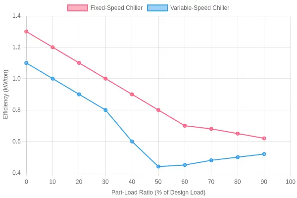
Figure 1. Fixed-speed vs. variable-speed chiller efficiency (kW/ton) across the part-load range. Variable-speed chillers hold their efficiency at part load, where real plants operate.
How to read this chart
- X-axis – Part-Load Ratio (% of Design Load): the share of the chiller’s rated (design) capacity actually being used at a given moment.
- Y-axis – Efficiency (kW/ton): the electrical power consumed per ton of cooling delivered. Lower is better: a lower number means less energy for the same cooling.
The two curves tell different stories:
| Part-Load Ratio | Fixed-Speed Chiller (kW/ton) | Variable-Speed Chiller (kW/ton) |
|---|---|---|
| 10% | 1.30 | 1.10 |
| 30% | 1.10 | 0.80 |
| 50% | 0.80 | 0.44 |
| 70% | 0.68 | 0.48 |
| 100% | 0.62 | 0.52 |
The fixed-speed chiller reaches its best efficiency only near full load. As the load falls, its efficiency collapses; at 10% load it burns more than double the energy per ton of its full-load rating. Because most real plants spend most of their hours between 30% and 60% load, this chiller operates much of its life well away from the point where it was rated.
The variable-speed chiller holds a much flatter curve, with its best efficiency around 50-60% load. The two curves separate most in the part-load region where buildings actually operate, and narrow to about 0.1 kW/ton at full load.
What this means for selection
Design-point efficiency for these two machines differs by roughly 0.1 kW/ton, yet their real-world operating costs diverge sharply. Part-load performance, not nameplate efficiency, determines the energy bill.
Turning Part-Load Behavior into Real Annual Operating Cost
A published kW/ton at design conditions is a single snapshot. Annual operating cost is the result of hundreds of hours at every load the plant actually sees. Load-weighted efficiency bridges the two.
The method is simple. Divide the year into part-load bands (say, 25%, 50%, 75%, and 100% of capacity). For each band you know the chiller plant part-load efficiency at that condition (kW/ton) and the number of annual hours the plant runs there. Compute a weighted average:
Load-weighted kW/ton = Σ (kW/ton_i × hours_i) / Σ hours_i
That figure is the efficiency the plant really achieves across the year. From it, annual energy use follows directly:
Annual kWh   = Load-weighted kW/ton × average tons × annual hours
Annual cost  = Annual kWh × blended utility rate
Why the design number lies
The discrepancy comes from where the hours land on the curve. Chillers rarely run at the design point; most of the calendar sits between 30% and 70% load. If that range falls on the flat, efficient part of the curve, the load-weighted value can come in below the design figure, and a design-point estimate will overstate cost. If the plant cycles often or runs heavily at low load – where staging, poor condenser conditions, and cycling losses push kW/ton up – the weighted value climbs above design, and the design figure badly understates the bill.
Cost scales linearly with kW/ton, so small distortions compound: a 0.15 kW/ton gap spread across hundreds of running hours and a large connected tonnage becomes a real line item.
Part-load weighting, not the nameplate rating, governs annual operating cost. Collect real load-duration data, bin it by efficiency band, and let the hours set the number you budget against.
Where the Hours Actually Land
If you want to know why design-condition efficiency rarely matches the energy bill, start with where the chiller spends its time. The doughnut chart below shows how annual operating hours typically divide across four part-load bands, as a share of total runtime.
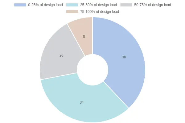
Annual chiller operating hours by part-load band (share of total runtime).
Reading the Bands
| Load Band | Share of Annual Hours | What It Means |
|---|---|---|
| 0-25% of design load | 38% | The single largest slice, and the band where many machines run least efficiently |
| 25-50% of design load | 34% | Combined with the lightest band, this is roughly three-quarters of all runtime |
| 50-75% of design load | 20% | Moderate load, closer to the efficient range for many chillers |
| 75-100% of design load | 8% | Design conditions are a small slice of real operation |
The point is hard to miss: about 72% of operating hours sit below 50% of design load. A chiller selected and rated at 100% load is therefore optimized for a condition it barely ever sees. The lightly loaded hours, where compressor cycling, low evaporator pressure, and poor part-load performance raise kWh per ton, dominate the calendar.
Why This Matters for Operators
A machine can pass its design-point acceptance test and still drain the budget month after month, because the efficiency curve sags exactly where the hours pile up. Facilities with variable occupancy – restaurants, mixed-use buildings, hospitality sites whose load swings from quiet afternoons to busy dinner service – live almost entirely in the low-load region. Managers tracking runtime through a BMS can check whether their own distribution leans even further toward the light bands.
For a practical illustration of how occupancy-driven load swings shape daily demand, see how a typical restaurant’s operating rhythm drives equipment cycling.
What Good Looks Like
- Measure, don’t assume. Log actual part-load hours before claiming an efficiency win.
- Weight IPLV, not just full-load kW/ton. Integrated part-load value reflects the weighted reality of the chart above.
- Right-size and stage. Multiple smaller chillers or variable-speed drives handle light loads far better than one large fixed-speed machine.
- Revisit controls. Reset strategies and condenser water optimization pay off most in the 0-50% bands.
Design conditions are a snapshot; operating hours are the record that matters.
Measuring and Monitoring Part-Load Performance in Practice
Design conditions tell you what a chiller can do on its best day. Monitoring tells you what it does across the thousands of hours it really runs. For facility managers and energy consultants, the goal is to turn trend data into a load-weighted efficiency profile that reflects hour-by-hour behavior rather than a single nameplate line.
Most of what you need already lives in the equipment you own. The work is capturing it consistently, cleaning it, and weighting it by load. The steps below quantify chiller plant part-load efficiency and connect it to real operating cost:
- Submeter each chiller to separate compressor power from pumps, towers, and auxiliary loads, then calculate kW/ton per machine rather than for the whole plant.
- Pull the part-load ratio from the chiller controller, ideally logged at one- or five-minute intervals so short cycling and staging events are not averaged away.
- Log entering and leaving evaporator temperatures to establish delivered tons of cooling, and entering and leaving condenser temperatures to capture the real lift the machine is fighting.
- Verify that condenser water reset is actually happening by trending supply setpoint against the programmed reset schedule, then flag hours where the setpoint stays flat while ambient or load conditions change.
- Export BMS trend data into a spreadsheet or analytics platform, bin the hours by load range, and weight each bin by runtime to build a load-weighted efficiency curve.
- Revisit the profile monthly and after any sequencing change. A curve that looked healthy last summer can flatten once a new tenant load reshapes the plant.
The payoff is a defensible number. Once you can show where hours are spent and what each bin costs per ton-hour, you can target the worst-performing load ranges first, tune sequencing and staging, and defend capital upgrades with data instead of assumptions. At that point part-load analysis stops being an exercise and starts showing up as a smaller utility bill.
Comparing Design-Point and Part-Load Energy Costs
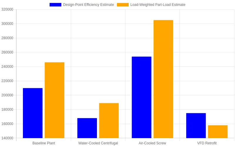
The chart places the two cost estimates side by side for four common plant scenarios. The blue bars are what you would predict from rated design-point efficiency; the orange bars are the more realistic figure once efficiency is weighted across the hours the plant runs. The gap between each pair is the money design conditions hide.
The gap moves in both directions:
| Scenario | Design-Point Estimate | Part-Load Estimate | Gap |
|---|---|---|---|
| Baseline Plant | $210,000 | $246,000 | +$36,000 |
| Water-Cooled Centrifugal | $168,000 | $189,000 | +$21,000 |
| Air-Cooled Screw | $254,000 | $305,000 | +$51,000 |
| VFD Retrofit | $175,000 | $158,000 | -$17,000 |
For the first three scenarios the part-load reality runs higher than the design-point promise, the classic understatement of operating cost. The air-cooled screw plant misses by the most, $51,000 a year, because its efficiency falls off steeply when mild weather drops the load. The VFD retrofit is the exception: part-load operation beats the design figure, which is why variable-speed control pays for itself.
When you compare chiller options, weight each machine’s efficiency against your building’s real load profile instead of trusting one rated number, and let the load-weighted column drive the decision.
Strategies to Improve Part-Load Efficiency
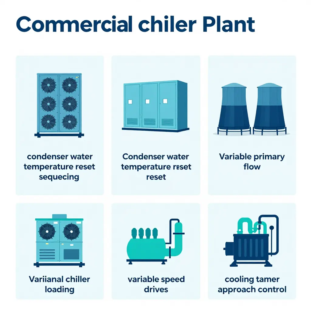
Most chillers spend the bulk of their running hours below design tonnage, so the choices you make for those in-between hours shape operating cost far more than nameplate numbers do. Improving chiller plant part-load efficiency rarely requires new equipment; it usually comes down to how well the plant is sized, sequenced, and controlled.
Right-Size and Sequence the Machines
A plant built around peak load usually runs at an awkward part load. When demand sits between stages, oversized machines short-cycle and waste energy on every restart. Match the smallest chiller to the building’s lowest sustainable load, then sequence units so one machine carries the base and others trim on as needed. Keep each running chiller loaded near its efficient range rather than barely alive.
Reset Condenser Water Temperature
Fixed condenser water temperatures are a design-condition habit. As outdoor wet-bulb temperatures fall, lower the condenser setpoint to cut compressor lift, so chillers do the same work with less power. A modest reset schedule that respects minimum flow and safe approach margins saves energy on almost every mild day.
Adopt Variable Primary Flow
Variable primary flow removes the fixed-speed bridge between production and demand. Varying evaporator flow with real load slows the pumps and cuts pump energy sharply during light-load hours. Pair it with accurate flow measurement and a stable minimum-flow strategy so chillers always see safe velocities.
Optimize Chiller Loading and Sequence
Instead of staging machines on and off at fixed thresholds, use an optimal-loading routine that distributes total tonnage across online chillers to reach the lowest combined kW. This is where the biggest part-load gains usually sit, because two lightly loaded machines are often cheaper than one heavily loaded unit.
Enable Variable-Speed Drives
Variable-speed drives on compressors, fans, and pumps let equipment follow load instead of running full-tilt against a throttle. Confirm the drives are enabled and tuned, and not bypassed by conservative controls or manual overrides left over from commissioning.
Keep Tower Approach Within Range
Cooling tower approach drives chiller efficiency more than most operators expect. If the tower cannot reach its design approach, the condenser runs warmer and compressor lift climbs. Clean fill, balanced airflow, and correct fan staging keep approach where it belongs, especially at part load, when towers are often neglected.
Tie the Strategy Together
Each measure helps on its own; combined under one plant-level optimization sequence, they compound. Facility teams and consultants who want a wider set of operational references can explore a broader informational resource like this sustainability and operations guide or a partner site’s collection of practical facilities notes. Measure real hours at load and reset setpoints as aggressively as safety allows, and the operating cost of the plant will reflect its actual duty rather than its design-day worst case.
FAQ: Part-Load Efficiency Questions Answered
Why is IPLV not the same as my chiller’s real operating efficiency?
Integrated Part Load Value (IPLV) is a single weighted number built from four standardized operating points, each with an assumed load percentage and condenser water temperature. Those assumptions rarely match how your plant runs, so a chiller with an excellent IPLV can still deliver poor real-world part-load efficiency. Treat IPLV as a tool for comparing equipment on paper, not as a prediction of your operating cost.
How is part-load ratio defined?
Part-load ratio (PLR) is the actual cooling load divided by the chiller’s rated capacity at that moment. A 500-ton chiller delivering 250 tons runs at a PLR of 0.5, or 50 percent. Tracked over time, PLR shows how many hours the plant spends at low, mid, and high load, which is where real part-load efficiency is decided.
Why do chillers rarely run at design conditions?
Design conditions represent the most demanding day the system was sized for, plus a safety margin. Real weather, occupancy, and internal loads change hour by hour, so most plants spend the bulk of their running hours below full load. Performance measured at design conditions therefore says little about the energy consumed in routine operation.
How can I measure part-load efficiency on an existing plant?
Meter chiller power (kW), delivered cooling (tons or kW), and condenser water temperature across different load ranges. Collect the data over several weeks, or ideally a full cooling season, to capture a representative range of conditions. Then calculate kW/ton or COP at each load band to build the plant’s real efficiency curve, and compare it against the design and IPLV figures.
Can part-load performance be improved without replacing chillers?
Yes, often substantially. Condenser water temperature reset, better chiller sequencing and staging, variable-speed drives, and eliminating low-delta-T syndrome can all lift part-load performance on existing equipment. Because most operating hours occur at partial load, these adjustments frequently cut operating cost with no capital replacement.